Inception, DenseNet, and the Efficiency Era

Inception: Why Choose One Filter Size? (2014)

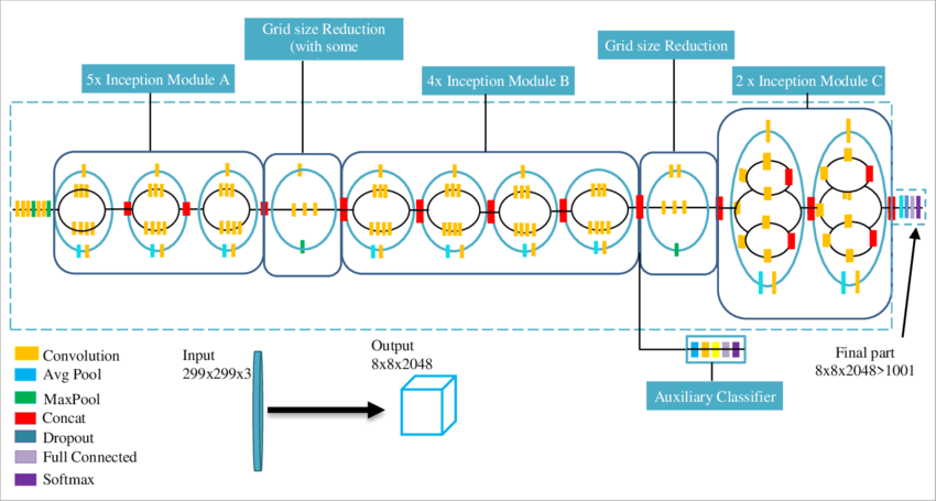
VGGNet committed to 3 × 3 filters everywhere. Inception (GoogLeNet) took a different philosophical stance: you do not have to choose a single filter size per layer. What if you applied multiple filter sizes in parallel and let the network decide which representations are useful?

An Inception module applies 1 × 1, 3 × 3, and 5 × 5 convolutions simultaneously, along with max pooling, and concatenates all the results along the channel dimension. The 1 × 1 convolutions serve as bottlenecks, reducing channel dimensionality before the more expensive 3 × 3 and 5 × 5 operations — a trick that makes the module surprisingly parameter-efficient.

The result: at the 2014 ILSVRC challenge, Inception achieved state-of-the-art results with 12× fewer parameters than AlexNet and better accuracy. This made it not just an academic success but a practical one — smaller models deploy faster and cheaper.

DenseNet: Every Layer Connected to Every Other Layer

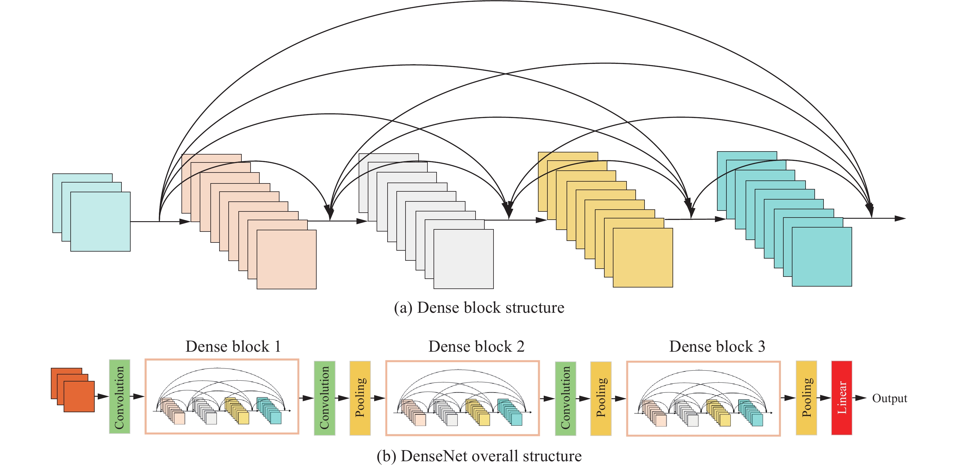
DenseNet takes the skip connection idea from ResNet and radicalizes it: every layer is connected to every other layer. In a network with L layers, there are L × (L+1) / 2 direct connections. Feature maps from layer 1 flow directly to layer 5. Feature maps from layer 3 flow directly to layer 7. All of them.

The benefits: alleviates vanishing gradient more aggressively than ResNet, and allows feature reuse throughout the entire network. The cost: significantly higher memory usage and a more complex hyperparameter landscape. DenseNet is powerful but demanding to train well.

SqueezeNet: Doing More With Less

SqueezeNet is a masterclass in efficiency. By introducing a "squeeze" layer (1 × 1 convolutions to reduce channels) followed by an "expand" layer (a mix of 1 × 1 and 3 × 3 convolutions), SqueezeNet achieves competitive accuracy with dramatically fewer parameters than AlexNet — making it particularly useful for deployment on resource-constrained devices.