Graph Neural Networks
What is a Graph?
A graph is a mathematical structure for representing relationships. Virtually any dataset where entities connect to other entities can be expressed as a graph: molecules, social networks, road maps, citation networks, and, as we'll see, user–item interactions in a recommender system.
Graphs let us move beyond tabular data. A table assumes each row is independent. A graph explicitly encodes the connections between rows, and those connections are often where the most useful information lives.


These examples span wildly different domains, but they all share the same underlying representation: a set of entities and a set of relationships between them.
Recommendation data is inherently relational: users interact with items, users follow other users, items belong to categories, and items share features. This structure maps naturally onto a graph, where users and items are nodes and interactions are edges.
Which of the following datasets is best represented as a graph rather than a flat table?
The Graph Data Structure
Formally, a graph is defined by three components:
- Vertices (nodes): The entities in the graph. Every node can carry a feature vector that describes it. In a molecule, a node might be an atom with features like atomic number, charge, and valence. In a recommender, a node might be a user with features like demographics and interaction history.
- Edges: The relationships between nodes. Edges can be directed (A → B, but not B → A) or undirected (A — B). Like nodes, edges can carry feature vectors. In a molecule, an edge (bond) might encode bond type (single, double, aromatic). In a recommender, an edge between a user and an item might encode the rating the user gave.
- Global attributes: A single feature vector attached to the entire graph, encoding properties that belong to the graph as a whole rather than to any individual node or edge. For a molecule, this might be the total molecular charge. For a social network, it might be the graph's diameter or overall density.
This three-level structure (nodes, edges, globals) means a graph can represent information at multiple scales simultaneously. A single graph object carries local information (individual node and edge features), relational information (which nodes are connected), and global context, all at once.
Click a node or edge to see its feature vector
Global attributes
Graph-level
| Graph type | Bipartite |
| Num. users | 3 |
| Num. items | 3 |
| Num. edges | 6 |
| Density | 66.7% |
| Avg. degree | 2.0 |
Explore the anatomy of a graph. Click any node to inspect its feature vector. Click any edge to see its attributes. The global attributes panel shows graph-level properties. Toggle between an example molecule and a small user–item interaction graph.


Graph Neural Networks
A GNN takes a graph as input and produces a graph as output. The output graph has the same connectivity as the input: the same nodes, the same edges, the same adjacency structure. A GNN does not add or remove nodes or edges.
What does change are the feature vectors attached to every node, edge, and the global attribute. The GNN updates these representations by passing messages between neighboring nodes and edges across multiple layers, so that by the final layer, each node's feature vector encodes not just its own attributes but also information about its local neighborhood and beyond.
Input graph → Output graph: same shape, richer features
If the input graph has 12 nodes and 18 edges, the output graph also has 12 nodes and 18 edges, described by the same adjacency list. The only thing the GNN changes is the content of the feature vectors at each node, edge, and the global attribute. You can think of it as the GNN "filling in" richer, context-aware representations while leaving the graph's skeleton intact.
The GNN achieves this through message passing. In each layer:
- Each node collects the feature vectors of its neighbors and aggregates them (e.g., by summing or averaging).
- The node combines this aggregated neighborhood signal with its own current feature vector to produce an updated representation.
- Edge and global representations are updated similarly: edges aggregate information from their endpoint nodes; the global attribute aggregates from all nodes and edges.
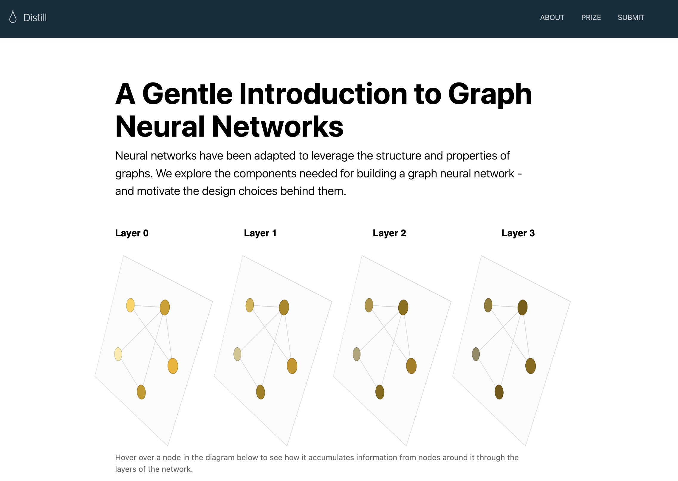
After L layers, a node's representation has been influenced by every node within L hops. A two-layer GNN lets information travel two steps across the graph; a three-layer GNN, three steps; and so on. This is how GNNs capture both local structure (immediate neighbors) and progressively more global structure (neighborhoods of neighborhoods).
After running a GNN on a graph with 50 nodes and 120 edges, the output graph has how many nodes and edges?
Recommendation Data as a Graph
Recommendation data is inherently relational: users interact with items, users follow other users, items belong to categories, and items share features. This structure maps naturally onto a graph, where users and items are nodes and interactions are edges.
Graph Neural Networks operating on this structure can propagate information between neighboring nodes, producing updated embeddings that encode local and global interaction patterns. This gives them a significant advantage over methods like PMF that treat users and items independently, with no notion of graph structure.

The User–Item Bipartite Graph
The simplest graph structure for collaborative filtering is a bipartite graph: one set of nodes represents users (U1, U2, …) and another set represents items (I1, I2, …). An edge between Ui and Ij indicates that user i has interacted with item j. Edge weights can encode interaction strength (e.g., a rating value or watch duration).
This structure encodes collaborative signals implicitly and elegantly:
- Two users who share many item neighbors are likely similar, and the GNN will learn to bring their embeddings close together.
- Two items that are connected to many of the same users are likely similar; again, the GNN captures this from graph structure alone, without requiring any item content features.

After GNN message passing, each user and item node has a rich embedding that reflects both its own attributes and the full context of its position in the interaction graph. Recommendations are then generated exactly as in PMF: compute dot-product similarity between a user embedding and all item embeddings, and return the top-K items.

The key difference from PMF: these embeddings encode multi-hop structural information. A user's embedding is shaped by the items they've interacted with, which are shaped by the other users who also interacted with them, which are shaped by their items, and so on across layers. This multi-hop propagation captures collaborative signals that a simple dot product of independently-learned embeddings cannot.
Live GNN playground: edit a molecule, adjust model hyperparameters (depth, aggregation, embedding sizes), and watch the model re-run inference in real time. The scatter plot shows PCA-projected graph embeddings across training epochs: each point is a molecule colored by its predicted pungency. Original visualization code by Sanchez-Lengeling, et al. and can be found here.
Distill · Research Article
A Gentle Introduction to Graph Neural Networks
"This article explores and explains modern graph neural networks."
Highly recommended reading that dives deeper into the theory of GNNs.