Evaluating Generative Models
Generative model evaluation is harder than discriminative model evaluation. There's no single accuracy number. We use a small constellation of metrics, each measuring something slightly different. Using only one is a mistake you'll see in weak papers — use all of them together.
Inception Score (IS)
Feed your generated images through a pretrained Inception network (the same Inception CNN from Computer Vision). For each image, the network outputs a probability distribution over classes. The Inception Score measures two things:
- Conditional distribution p(y|x): for any individual generated image, the classifier should be confident about which class it depicts. A clear cat photo gets a peaked distribution. High confidence = low entropy in p(y|x).
- Marginal distribution p(y): averaged over all your generated images, the classifier should see a variety of classes. Diverse outputs = high entropy in p(y).
IS = exp(E[]). Higher IS = better.
Known limitation: IS is calculated only from generated images, never comparing them to real images. A generator that produces 1000 different cleanly-classifiable classes will score well even if those images look nothing like the real training distribution.
Each image gets its own probability distribution from Inception
Feed each generated image into Inception. For every image individually, the network outputs a confidence score for each class — this is p(y | x), read as "the probability of class y, given this specific image x." Click any image to see its distribution.
p(y | x) for image 1 — "given this image, what class is it?"
Inception is confident about this image — one class dominates. This is good for IS.
Average all images together to get the overall distribution
Now average the per-image distributions across all generated images. The result — p(y), "the probability of class y overall" — tells you how varied the generator's output is. If it only ever makes cats, p(y) will be almost entirely "cat."
p(y) — averaged across all 5 images — "how varied is the output?"
Spread evenly across all classes — the generator is diverse. High entropy = good.
Measure how different each image's distribution is from the average
For each image, compute how much its p(y|x) diverges from p(y) using KL divergence. A clear cat photo has a very different distribution from the flat average — large KL. Average those KL values, then exponentiate to get IS. Higher IS = more confident and more diverse.
| Image | p(y|x) peaks at | KL( p(y|x) ‖ p(y) ) |
|---|---|---|
| 🐱 image 1 | 🐱 cat (90%) | 1.126 |
| 🐶 image 2 | 🐶 dog (88%) | 1.078 |
| 🚗 image 3 | 🚗 car (85%) | 1.012 |
| 🐦 image 4 | 🐦 bird (91%) | 1.152 |
| 🐟 image 5 | 🐟 fish (87%) | 1.056 |
| Average KL — E[ KL(p(y|x) ‖ p(y)) ] | 1.085 | |
IS = exp( 1.085 )
High — images are confident (peaked p(y|x)) and diverse (spread p(y)).
IS
2.96
IS blind spot
IS only looks at generated images. It never compares them to real data. A model that generates crisp, classifiable images of 1,000 different entirely fictional objects would score high even if none of them resemble a real photograph. That is why FID was invented.
Walk through how IS is calculated step by step. Switch between scenarios to see how confidence and diversity each affect the score.
Fréchet Inception Distance (FID)
FID addresses IS's weakness by comparing generated images to real images directly. We pass both real and generated images through Inception, take feature vectors from an intermediate layer (typically pool3), and model the resulting feature distributions as multivariate Gaussians with means μ and covariance matrices Σ. Then:
where subscript 1 is real images, subscript 2 is generated images, and Tr is the trace (which condenses a matrix to a scalar). Lower FID = better.
Why FID is more trustworthy than IS:
- Compares to real images directly
- Captures covariance structure (shapes, textures, object relationships), not just means
- Compares features, not raw pixels — aligns better with human perception
- The de facto standard metric in modern generative image research
Pass both real photos and generated images through Inception — but instead of reading the final class probabilities, stop one layer earlier and grab the raw feature vector (the pool3 layer, 2048 dimensions). Each image becomes a point in feature space. This 2D plot represents that space.
The orange (generated) and blue (real) clouds overlap well — the features look similar.
Why features instead of pixels?
Raw pixels are just numbers — two images can differ wildly in pixel values while looking nearly identical to a human. Inception features capture high-level structure: shapes, textures, objects. Comparing feature distributions is much closer to how humans judge image quality.
Walk through how FID is calculated step by step. Switch between scenarios to see how each affects the feature distributions and the final score.
Reconstruction Error (for VAEs)
Because a VAE both encodes and decodes, we can measure how well it reconstructs its inputs. Lower reconstruction error means the model captures important features of the data in its latent space. Common formulations:
- MSE (Mean Squared Error) — emphasizes large pixel deviations
- MAE (Mean Absolute Error) — more robust to outliers
- Binary Cross-Entropy — common for image data with normalized pixel values in [0, 1]
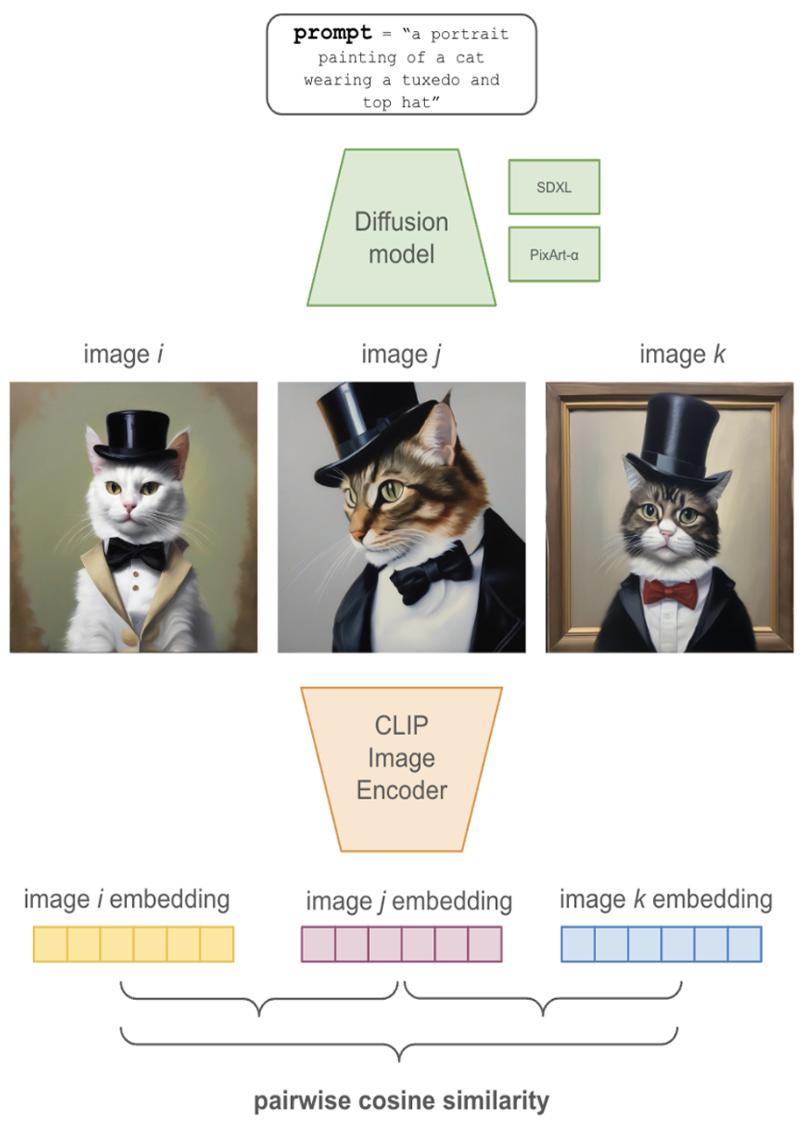
Semantic Similarity (for Diffusion Models)
Diffusion models are stochastic — feed in the same prompt twice and you get two different images. Sometimes that's wonderful (creative variety) and sometimes that's bad (you need consistency for a brand campaign). Semantic similarity quantifies how consistent a model's outputs are:
- Take a set of prompts.
- Generate many images for each prompt.
- Embed every image with CLIP.
- Compute pairwise cosine similarity across all embeddings.
- Average them.
Scores between 0 and 100. Higher = more consistent. Choose based on whether you want a workhorse that produces consistent outputs or a creative model that gives you wild variety.
A researcher generates 10,000 images using a GAN trained on ImageNet. The images are all perfectly crisp and clearly classifiable, but they look nothing like real photographs — they have an unnatural synthetic aesthetic. Which metric would catch this problem?